Calculate the regret of a strategy in individual states and across states
Calculate a strategy’s satisficing robustness
Visualize different robustness for various metrics and strategies in insightful ways
Demonstrate your conceptual understanding of the two robustness criteria from the study
(Optional) Apply the workflow to your project data
Lab Workflow
Repository Setup
You can call the repository rdm_lab/.
If you need a reminder on how to set up your project directory and create a GitHub repository, check the workflow and directory structure from lab 2.
You can directly export these lab instructions as a .ipynb file (look at the top right of the page). Place this file in the noteboks/ subdirectory.
Environment Setup
For today’s lab, you will need to create an environment that has all the packages from lab 2, plus scipy.
Be sure to include instructions in your README.md about how others can prepare the computational environment to run your notebook.
Our Analysis
Make sure your environment is set up and active to run the code cells below.
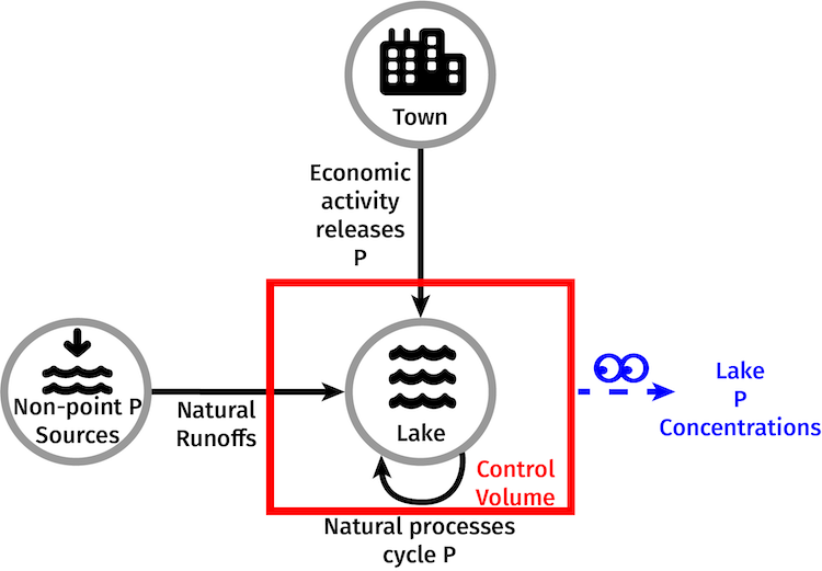
Lake Problem Overview
Quoting from Lempert and Collins (2007): “Imagine a small village perched on the shores of a pristine lake. Many of the town’s citizens want economic development, but development will increase the pollution flowing into the lake. The citizens know that lakes such as theirs can exhibit a threshold behavior where a small pollution increase past some level may cause a clear lake to turn suddenly and sometimes irreversibly cloudy. The citizens seek a development plan that preserves the clarity of their lake, cognizant of their widely divergent values regarding environmental quality and growth, as well their divergent opinions about the level where the pollution threshold for their lake might lie. The town’s citizens also know that once permits are issued, buildings built, and pollution begins to flow it may become difficult to reverse course. Nonetheless, they must decide how much pollution they should allow to best balance their economic and environmental goals.”
The lake naturally loses and gains phosphorus (P). The lake can exist in one of two states. The desirable state, called an oligotrophic state, exists with low nutrient inputs, low to moderate levels of plant production, and relatively clear water. The undesirable state, called an eutrophic state, exists with high nutrient levels, high levels of plant production, low biodiversity, and murky water. The introduction of economic activity to the lake increases the risk of eutrophication.
Lempert and Collins (2007) represent the lake problem with the following equation (with a little clarification from revisiting Peterson et al., (2003)): \[
X_{t+1} =
\begin{cases}
BX_t + b_t + L_t & \text{if } X_t < X^{\text{crit}} \\
BX_t + r + b_t + L_t & \text{if } X_t \geq X^{\text{crit}}
\end{cases}
\]
where \(X_{t}\) is the P concentration at time \(t\), \(B\) is the proportion of P retained in the lake each year, \(b_{t} = (\bar{b}, \omega)\) is the natural pollution flow into the lake assumed to follow a normal distribution with mean \(\bar{b}\) and standard deviation \(\omega\), \(L_{t}\) is the anthropogenic pollution flow, and \(r\) is the amount of P recycled and maintained in the lake. \(X^{\text{crit}}\) is the critical P concentration at which P recycling begins.
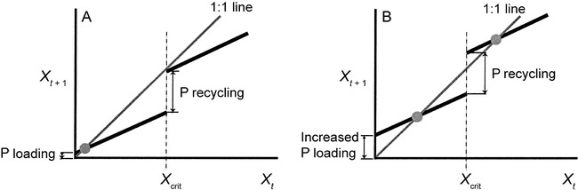
The two alternating equilibrium values are found by letting \(X_{t+1} = X{t}\):
If \(X_{1*} < X^{\text{crit}}\) an oligotrophic equilibrium exists, and if \(X_{2*} \geq X^{\text{crit}}\) a eutrophic equilibrium also exists. Because the equilibrium value of \(X\) depends upon the P loading, changes in P loading can cause equilibrium point to appear or disappear. Figure 2 from Peterson et al., (2003), shown below, illustrates how changes in P loading can irreversibly alter the lake system’s outcomes:
An illustration of the P dynamics model. In example (A), low P loading results in a single stable oligotrophic equilibrium. In (B), at a higher P loading the same lake has two stable equilibrium values—one oligotrophic (the lower point) and one eutrophic (the higher point)
Lempert and Collins (2007) assume that the citizens of the town gain utility by adding pollutants to the lake, but suffer a loss of utility if the lake becomes eutrophic. They represent the utility function as:
where \(\alpha\) and \(\beta\) are constants. \(\beta >> \alpha L_{t}\), representing that the loss of utility in the eutrophic state (e.g., recreational and aesthetic utility) is large compared to the utility gained from pollution. The citizens also may suffer economic losses, such as costs of retrofitting infrastructure with pollution control equipment or underutilization of capital stock, if they are forced to decrease emissions below their previously allowed level. These costs are small compared to those of the eutrophic state, given by:
where \(\varphi\) is a constant and \(\varphi << \frac{\beta}{L_{t-1} - L_{t}}\).
The town’s decision problem is to choose a pollution series, \(\mathbf{L_t}\),
Lempert and Collins propose a policy rule that has three decision variables: the initial level of pollution, \(L_{0}\), the max amount of pollution per time period, \(\Delta L\), and a safety margin, \(S\). This decision strategy takes the following form:
and \(\langle X^{\text{crit}}_{t} \rangle\) is the town’s estimated critical threshold at the current time period. Please refer to the paper for the formulation.
Under an expected utility maximization framework for decision-making, the town aims to maximize the present value of utility: \(PV(U) = \sum_{t} \frac{U_{t}}{(1 + d)^{t}}\), where \(d\) is the citizens’ discount rate. Given the available information to estimate \(\langle X^{\text{crit}}_{t} \rangle\), the town can find the optimal values for their decision variables. As we’ll see later in the lab (and as you already know from reading the paper), whether this is the right decision to make depends on how much you believe the information you have to estimate \(\langle X^{\text{crit}}_{t} \rangle\).
The basecase values of model parameters are as follows:
Parameter
Value
Retained phosphorous (B)
.2
Mean of natural emissions (\(\hat{b}\))
.1
Initial P concentration (\(X_{0}\))
\(\hat{b}\)/(1 - B) = .125
Std of natural emissions \(\omega\)
.04
Recycling rate (r)
.25
Std of measured \(X^{\text{crit}}\) (\(\gamma\))
.05
Distance from \(X^{\text{crit}}\) required for learning (\(\lambda\))
.1
Noise exponent (q)
2
Initial estimate of observed \(X^{\text{crit}}\) variance
.02
Discount rate (d)
.03
Utility from pollution (\(\alpha\))
1
Eutrophic cost (\(\beta\))
10
Emissions reduction cost (\(\varphi\))
1
Note: While the table in the text has \(\varphi\) as 10, the text clearly states that this emissions reduction cost is much smaller than the eutrophic cost so it is a typo. I’m guessing it’s supposed to be 1 (similarly, the initial estimate of observed \(X^{\text{crit}}\) variance is a typo in the paper’s table).
Decision-making under uncertainty
Note that I was not able to reproduce the results from Lempert and Collins completely. There are a few typos (e.g., see their Table on parameter values and the reported initial estiamte of observed \(X_{\text{crit}}\) and the one I was able to update based on other text in the paper). There are a few decisions and implementation choices I can’t back out without more guidance, but I was able to reproduce the most relevant behavior of the inflows and policies. I made a few updates relative to the policy rules as written in the manuscript:
I estimate the new best guess for \(X_{\text{crit}}\) based on the current best guess for variance. The notation as currently written suggests we calculate the new variance before updating our mean estimate.
I limit updates on standard deviation of \(X_{\text{crit}}\) to double our intial guess. If we don’t do this, there is too much noise in early draws and we can’t identify when our initial guess is lower than \(X^{\text{true}}_{\text{crit}}\). I think this biases our representation a bit more towards trusting our priors than the Lempert and Collins paper, but I can’t otherwise figure out how to get the same learning behavior as them for Strategy A when \(X^{\text{true}}_{\text{crit}}\) = .9.
Anyone who wants to review the paper and code and reconcile any major differences with explanations or code updates is more than welcome!
Because the code below does reproduce key behavior of the inflows and policies, all of the lessons about robustness are the same and that’s the key point of this lab.
Ok! Moving on…
Adapting the narrative of Lempert and Collins slightly, suppose the town reviewed scientific evidence of nearby lakes and concludes that \(X_{\text{crit}}\) lies between .3 and .9. The current best evidence suggets \(X_{\text{crit}} \sim N(.8, .138)\).
If the town has 100% confidence in this belief, the optimal strategy (called Strategy A) has: \(L_{0} = .31\), \(\Delta L = .027\)\(S = 2.8\)
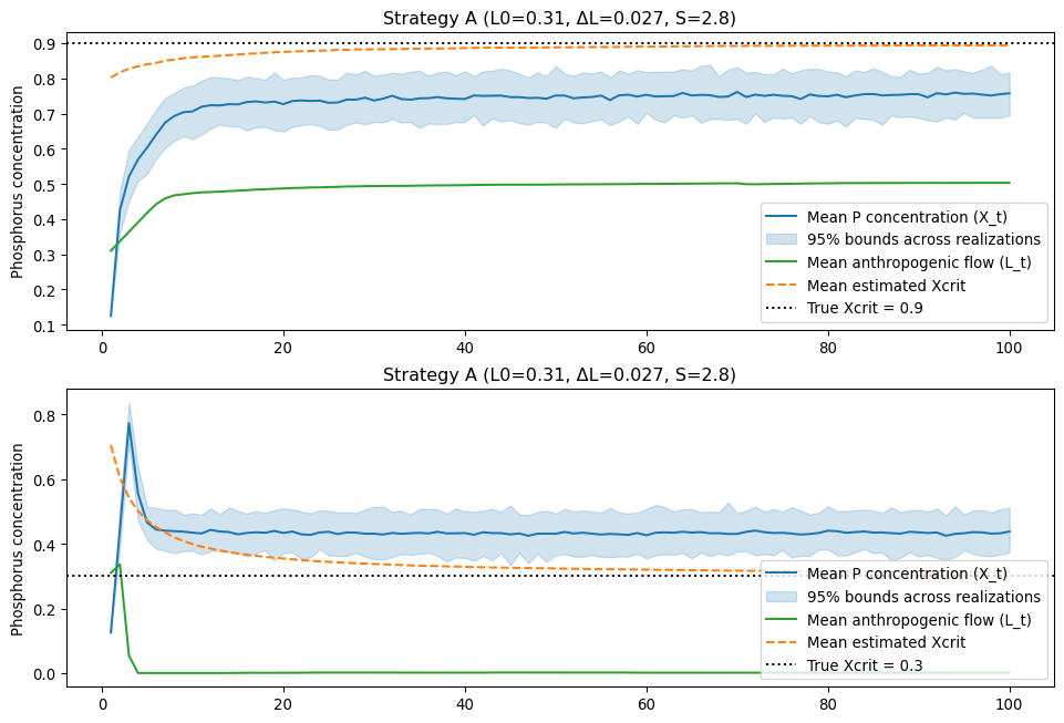
Assume that the true value of \(X_{\text{crit}}\) is .9. What does the pollution concentration of the lake look like over 100 years? What about if the true value is .3?
Code
import mathimport numpy as npfrom scipy.stats import truncnormimport matplotlib.pyplot as pltimport seaborn as sns# ------------------------# Parameters (Table I / paper)# ------------------------B =0.20# retained phosphorusb_bar =0.10# mean natural emissionsomega =0.04# std dev natural emissionsr =0.25# recycling jump when X >= Xcritgamma_obs =0.05# baseline observation noise stdlambda_learn =0.10q_noise =2.0initial_var =0.02alpha =1.0beta =10.0phi =1.0# table says 10 but the text says << betadiscount_rate =0.03# Strategy A (given)strategy_A = {"L0": 0.31, "dL": 0.027, "S": 2.8}# Simulation controlsT =100# yearsNsim =100# ensemble size for mean / quantiles (set e.g., 100 for demo)SEED =42rng_global = np.random.default_rng(SEED)# Initial estimate used by the towninitial_est_mean =0.787initial_est_var = initial_varest_lower =.3est_upper =.9# ------------------------# Helper functions implementing paper's learning and policy rules# ------------------------def gamma_t_func(Xt, Xcrit_true, gamma=gamma_obs, lam=lambda_learn, q=q_noise):"""Equation (6): observation noise depends on proximity to threshold."""if Xt >= Xcrit_true:returnfloat(gamma) exponent = ((Xcrit_true - Xt) / lam) ** qreturnmin(gamma * math.exp(exponent), .1) def kalman_update(mean_prev, var_prev, Zt, gamma_t):"""Scalar Kalman-like update (Equation (5))""" K = var_prev / (var_prev + gamma_t) mean_new = mean_prev + K * (Zt - mean_prev) var_new = (var_prev * gamma_t) / (var_prev + gamma_t)return mean_new, var_newdef target_emission_level(estimated_Xcrit, Xt, Xcrit_true, S):"""Equation (8) for L_target"""if Xt < Xcrit_true: target = (1.0- B) * estimated_Xcrit - b_bar - S * omegaelse: target = estimated_Xcrit - B * Xt - r - b_bar - S * omegareturnmax(0.0, target)def next_L(Lt, L_arg, dL):"""Equation (7) update for L"""returnmax(0.0, min(Lt + dL, L_arg))def simulate_one_run_with_learning(Xcrit_true, policy, T=100, rng=None, est_mean_init=initial_est_mean, est_var_init=initial_est_var):""" Simulate one stochastic run with Kalman learning and the adaptive policy (L0, dL, S). Returns time series dict with keys: X, L, est (estimated Xcrit), U (period utilities) """if rng isNone: rng = np.random.default_rng() L0 =float(policy["L0"]) dL =float(policy["dL"]) S =float(policy["S"]) X = np.empty(T) L = np.empty(T) Z = np.empty(T) est = np.empty(T) U = np.empty(T) Xt = b_bar / (1.0- B) # initial concentration per paper L_prev = L0 L_curr = L0 est_mean = est_mean_init est_var = est_var_initfor t inrange(T):# natural inflow bt = rng.normal(b_bar, omega)# update concentration (Eqn 1)if Xt >= Xcrit_true: Xt_next = B * Xt + r + bt + L_currelse: Xt_next = B * Xt + bt + L_curr# observation for learning: Zt ~ N(Xcrit_true, gamma_t) gamma_t = gamma_t_func(Xt, Xcrit_true) Zt = rng.normal(loc=Xcrit_true, scale=gamma_t)# Kalman update est_mean, est_var = kalman_update(est_mean, est_var, Zt, gamma_t)# utility for this period (using current Xt and current emissions L_curr) reduction_cost = phi *max(0.0, L_prev - L_curr) eutrophic_penalty = beta if Xt >= Xcrit_true else0.0 U[t] = alpha * L_curr - reduction_cost - eutrophic_penalty# record X[t] = Xt L[t] = L_curr est[t] = est_mean# compute target and update emissions L_targ = target_emission_level(est_mean, Xt, Xcrit_true, S) L_next = next_L(L_curr, L_targ, dL) L_prev = L_curr L_curr = L_next Xt = Xt_nextreturn {"X": X, "L": L, "est": est, "U": U}# ------------------------# Run simulation # ------------------------all_X = np.zeros((Nsim, T))all_L = np.zeros((Nsim, T))all_est = np.zeros((Nsim, T))all_U = np.zeros((Nsim, T))all_X2 = np.zeros((Nsim, T))all_L2 = np.zeros((Nsim, T))all_est2 = np.zeros((Nsim, T))all_U2 = np.zeros((Nsim, T))# True Xcrits for this illustrationxcrit_list = [0.3, 0.4, 0.5, 0.6, 0.7, 0.8, 0.9]n_x =len(xcrit_list)# pre-allocate arrays: shape (n_x, Nsim, T)all_X = np.zeros((n_x, Nsim, T))all_L = np.zeros((n_x, Nsim, T))all_est = np.zeros((n_x, Nsim, T))all_U = np.zeros((n_x, Nsim, T))# Pre-generate natural inflows bt_samples for each Monte Carlo run (CRN across Xcrit)rng_global = np.random.default_rng(SEED)bt_samples = rng_global.normal(loc=b_bar, scale=omega, size=(Nsim, T))# Run ensemblefor i inrange(Nsim):# create per-run rng for observation draws (do not re-seed inside loop) rng_i = np.random.default_rng(SEED +1000+ i)for j, xcrit inenumerate(xcrit_list): out = simulate_one_run_with_learning(Xcrit_true=xcrit, policy=strategy_A, T=T, rng=rng_i, est_mean_init=initial_est_mean, est_var_init=initial_est_var) all_X[j, i, :] = out["X"] all_L[j, i, :] = out["L"] all_est[j, i, :] = out["est"] all_U[j, i, :] = out["U"]# ------------------------# Plot results: mean concentration, emissions, and estimated Xcrit# ------------------------years = np.arange(1, T+1)fig, ax = plt.subplots(2, 1, figsize=(12, 8))# Top: concentration and estimated thresholdax[0].plot(years, all_X[-1].mean(axis=0), color="C0", label="Mean P concentration (X_t)")ax[0].fill_between(years, np.percentile(all_X[-1], 5, axis=0), np.percentile(all_X[-1], 95, axis=0), alpha=.2, color="C0", label="95% bounds across realizations")ax[0].plot(years, all_L[-1].mean(axis=0), color="C2", label="Mean anthropogenic flow (L_t)")ax[0].plot(years, all_est[-1].mean(axis=0), color="C1", linestyle="--", label="Mean estimated Xcrit")ax[0].axhline(xcrit_list[-1], color="k", linestyle=":", label=f"True Xcrit = {xcrit_list[-1]}")ax[0].set_ylabel("Phosphorus concentration")ax[0].set_title("Strategy A (L0=0.31, ΔL=0.027, S=2.8)")ax[0].legend()ax[1].plot(years, all_X[0].mean(axis=0), color="C0", label="Mean P concentration (X_t)")ax[1].fill_between(years, np.percentile(all_X[0], 5, axis=0), np.percentile(all_X[0], 95, axis=0), alpha=.2, color="C0", label="95% bounds across realizations")ax[1].plot(years, all_L[0].mean(axis=0), color="C2", label="Mean anthropogenic flow (L_t)")ax[1].plot(years, all_est[0].mean(axis=0), color="C1", linestyle="--", label="Mean estimated Xcrit")ax[1].axhline(xcrit_list[0], color="k", linestyle=":", label=f"True Xcrit = {xcrit_list[0]}")ax[1].set_ylabel("Phosphorus concentration")ax[1].set_title("Strategy A (L0=0.31, ΔL=0.027, S=2.8)")ax[1].legend(loc='lower right')
When the neighboring lakes’ statistics are represenative of the town’s lake (top panel, true Xcrit = 0.9), Strategy A lets emissions ramp up and stabilizes at a moderate level that keeps the mean phosphorus concentration under the town’s safety buffer. When the assessment is badly wrong (bottom panel, true Xcrit = 0.3), the initial policy overcommits — the emissions (and then concentration) rise, the town’s estimate of \(X_{\text{crit}}\) is revised downward as observations arrive, and emissions are sharply cut only after the system has already been driven into the eutrophic equilibrium. This illustrates how a predict‑then‑act rule that trusts a single prior can be fragile under deep uncertainty.
How much would the town regret going with Strategy A if \(X^{\text{true}}_{\text{crit}}\) = .3?
To estimate this, we are going to consider the town’s uncertainty about their estimate of the value of \(X_{\text{crit}}\) as well as epistemic uncertainty about whether this is the correct distribution to characterize \(X_{\text{crit}}\).
Recall from lecture that the regret of action a in state x is:
the difference between the present value expected utility of the optimal action in a considered state of the world and the considered action’s present value expected utility in that state of the world.
Considering the probability distribution \(p_{i}(x)\) over possible states of the world, the expected regret of action a on distribution i is:
I use actions, a, as opposed to strategies in this formulation because it is consistent with the original derivation in Savage (1951). Otherwise, the notation is consistent with the formulation in Lempert and Collins. x refers to the possible values for \(X_{\text{crit}}\) and i refers to a specific prior distribution for \(X_{\text{crit}}\).
For different values of \(X_{\text{crit}}\), we can estimate the town’s expected regret for placing all of their trust in the commissioned science assessment. Lempert and Collins provide several other strategies, B-G. For different values of \(X_{\text{crit}}\), we can calculate which of the strategies A-G is optimal and then calculate the expected regret of choosing Strategy A based on the town’s prior distribution for A. Lempert and Collins presumably identify the optimal strategy for each \(X_{\text{crit}}\) and calculate regret based on that, but we are just going to use the strategies provided to simplify things.
We’ll start with the example of \(X_{\text{crit}}\) = .3, which corresponds to the bottom panel of the figure we generated above. At \(X_{\text{crit}}\) = .3, Strategy G is optimal out of the strategies under consideration. Lempert and Collins don’t report the decision variables for this strategy, but we can get a very similar strategy to G by looking at Figure 6. It looks like \(L_{0} = 0.01\), \(\Delta L = 0.01\) and \(S = 5.8\).
We’ll build up slowly to expected regret over a prior distribution by first calculating the regret of Strategy A in the scenario where \(X_{\text{crit}}\) = 0.3. We need to calculate:
\(R_{A}(0.3) = PV(U_{G}(0.3)) - PV(U_{A}(0.3))\)
We’ll calculate the expected present value of utility of each strategy when \(X_{\text{crit}}\) = .3 and then the difference.
Code
# Strategy G (guessed from Fig. 6)strategy_G = {"L0": 0.01, "dL": 0.01, "S": 5.8}# Create the utility array for strategy Gstrat_g_U = np.zeros((n_x, Nsim, T))# Run ensemble for Strategy Gfor i inrange(Nsim):# create per-run rng for observation draws (do not re-seed inside loop) rng_i = np.random.default_rng(SEED +1000+ i)for j, xcrit inenumerate(xcrit_list): out = simulate_one_run_with_learning(Xcrit_true=xcrit, policy=strategy_G, T=T, rng=rng_i, est_mean_init=initial_est_mean, est_var_init=initial_est_var) strat_g_U[j, i, :] = out["U"]# Compute present value of utility.# Discount factors (length T)t = np.arange(T)discount_factors =1.0/ ((1.0+ discount_rate) ** t)pv_A_samples = np.sum(all_U[0, :, :] * discount_factors, axis=1) pv_G_samples = np.sum(strat_g_U[0, :, :] * discount_factors, axis=1)# Calculate expected values and report both and differencemean_pv_A = pv_A_samples.mean()mean_pv_G = pv_G_samples.mean()g_best_regret = mean_pv_G - mean_pv_Aprint("Strategy A: mean PV = {:.2f}".format(mean_pv_A))print("Strategy G: mean PV = {:.2f}".format(mean_pv_G))print(" Regret = {:.2f}".format(g_best_regret))
Strategy A: mean PV = -310.81
Strategy G: mean PV = -17.38
 Regret = 293.43
And we can do the same for when \(X^{\text{crit}}\) = .9 but this time we treat Strategy A as the optimal policy.
Code
# Compute present value of utility.# Discount factors (length T)t = np.arange(T)discount_factors =1.0/ ((1.0+ discount_rate) ** t)pv_A_samples = np.sum(all_U[-1, :, :] * discount_factors, axis=1) pv_G_samples = np.sum(strat_g_U[-1, :, :] * discount_factors, axis=1)# Calculate expected values and report both and differencemean_pv_A = pv_A_samples.mean()mean_pv_G = pv_G_samples.mean()a_best_regret = mean_pv_A - mean_pv_Gprint("Strategy A: mean PV = {:.2f}".format(mean_pv_A))print("Strategy G: mean PV = {:.2f}".format(mean_pv_G))print(" Regret = {:.2f}".format(a_best_regret))
Strategy A: mean PV = 15.24
Strategy G: mean PV = 7.27
 Regret = 7.98
Criterion 1: trading-off optimality for less sensitivity to unverifiable assumptions
How do we reconcile the differences in present value expected utility and expected regret? Lempert and Collins define a robust strategy as one that will have a smaller value of the weighted average of the best and worst case regrets compared to the strategy that optimizes expected utility, which we can represent as:
where \(0 \leq z \leq 1\) and represents our belief in \(p_{\text{best}(x)}\).
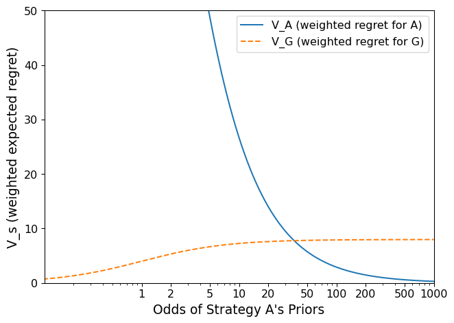
When \(z\) = 1, there is only one probability distribution under consideration - the town’s best guess. In this case, the equation above preserves the ordering of strategies produced by an expected utility calculation. When \(z\) = 0, the criterion is equivalent to avoiding worst-case utility. When \(z\) is in between, it is possible to identify the strategy that minimizes expected regret as a function of a decisionmaker’s odds that the initial probability distribution is correct (Fig. 7 in the paper). The odds are \(\frac{z}{(1-z)}\).
How confident does the town have to be in the scientific assessment to stick with Strategy A? To do this, we’ll calculate \(V_{s}\) for strategies A and G over a wide range of values for \(z\). Since we are only considering strategies A and G:
\(\bar{R}_{A, \text{best}}\) is 0, \(\bar{R}_{A, \text{worst}}\) is the regret we calculated when \(X_{crit}\) = 0.3, \(\bar{R}_{G, \text{best}}\) is the regret we calculated when \(X_{crit}\) = 0.9, and \(\bar{R}_{G, \text{worst}}\) is 0.
Code
# Calculated V_sdef weighted_regret(z, best_regret, worst_regret):return z*(best_regret) + (1-z)*(worst_regret)# Odds from 0.01 to 100# Construct odds grid (log-spaced) and convert to z = odds/(1+odds)odds = np.logspace(-2, 3, 500)z_list = odds / (1.0+ odds)# Calculate V_A and V_G over oddsV_A = z_list *0+ (1- z_list) * g_best_regretV_G = z_list * a_best_regret + (1- z_list) *0# Plot odds against weighted regretfig, ax = plt.subplots()ax.plot(odds, V_A, label='V_A (weighted regret for A)', linestyle='-')ax.plot(odds, V_G, label='V_G (weighted regret for G)', linestyle='--')ax.set_ylabel("V_s (weighted expected regret)", size=14)ax.set_xscale('log')# integer ticks to show (only those within the odds range will be used)integer_ticks = [1, 2, 5, 10, 20, 50, 100, 200, 500, 1000]# Choose x limits: show more of odds > 10 — e.g., start at 0.1 to include small odds tooax.set_xlim(0.1, 1000)# Keep only ticks that fall inside the x limitsticks_in_range = [t for t in integer_ticks if (t >= ax.get_xlim()[0] and t <= ax.get_xlim()[1])]ax.set_xticks(ticks_in_range)# Label ticks as integers (no decimals)ax.set_xticklabels([str(int(t)) for t in ticks_in_range])ax.set_xlabel("Odds of Strategy A's Priors", size=14)ax.set_ylim([0, 50])ax.tick_params(labelsize=12)ax.legend(fontsize='large')fig.tight_layout()
Based on this figure and fig. 7 in the paper, we can make a few observations about robust decision-making with this criterion. First, because of how poorly strategy A performs under low \(X^{true}_{crit}\), the town should be very confident in the scientific assessment to go with strategy A. Second, having more strategy options (fig. 7 in the paper) can help decisionmakers make more robust decisions under a wide range of beliefs.
Criterion 2: performing well over a wide range of plausible futures
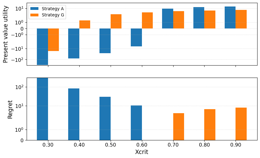
We’ll now shift our attention to a second robustness criterion: satisficing over a wide range of futures. While decisionmakers may want to identify satisficing strategies over multiple objectives, Lempert and Collins use regret for this criterion. This translates to finding a strategy that has low regret for many values of \(X^{true}_{crit}\). In the paper, they define arbitrary cutoffs for what constitutes “good enough” regret. In practice, analysts and decisionmakers often iterate on defining a satisficing threshold based on visualizations about strategy performance over a wide range of futures and refined sets of strategies.
We’re going to consider both the net present value of expected utility and regret for strategies A and G.
Code
# Helpful for getting the pv for multiple xcritdef compute_pvs_from_U(U_array, discount_rate): U = np.asarray(U_array) t = np.arange(U.shape[2]) discount_factors =1.0/ ((1.0+ discount_rate) ** t) pv = (U * discount_factors).sum(axis=2) return pvpv_A_samples = compute_pvs_from_U(all_U, discount_rate) pv_G_samples = compute_pvs_from_U(strat_g_U, discount_rate) # Mean present value over each xcrit# Same index as all_U and strat_g_Umean_pv_A = pv_A_samples.mean(axis=1) mean_pv_G = pv_G_samples.mean(axis=1) # Calculate regret# Two strategies under consideration, so regret is# 0 when one of the strategies is better for a xcrit valuepv_best_by_x = np.maximum(mean_pv_A, mean_pv_G) regret_A = pv_best_by_x - mean_pv_Aregret_G = pv_best_by_x - mean_pv_G# Plot regret over critical x values in one panel# Plot present value expected utility in the other# x values (e.g., xcrit_list)x = np.array(xcrit_list)n_x =len(x)# bar width and positionswidth =0.35xpos = np.arange(n_x)fig, ax = plt.subplots(nrows=2, sharex=True, figsize=(10,6))# Top: expected PV barsax0 = ax[0]ax0.bar(xpos - width/2, mean_pv_A, width=width, color='C0', label='Strategy A')ax0.bar(xpos + width/2, mean_pv_G, width=width, color='C1', label='Strategy G')ax0.set_ylabel('Present value utility', size=14)ax0.legend()ax0.grid(axis='y', linestyle=':', alpha=0.6)# Bottom: regret barsax1 = ax[1]ax1.bar(xpos - width/2, regret_A, width=width, color='C0')ax1.bar(xpos + width/2, regret_G, width=width, color='C1')ax1.set_ylabel('Regret', size=14)ax1.grid(axis='y', linestyle=':', alpha=0.6)# x ticks and labelsax1.set_xticks(xpos)ax1.set_xticklabels([f"{val:.2f}"for val in x])ax1.set_xlabel('Xcrit', size=14)ax[0].set_yscale('symlog')ax[1].set_yscale('symlog')ax0.tick_params(labelsize=12)ax1.tick_params(labelsize=12)
This kind of visualization helps put into context the relative performance of the strategies for different scenarios of \(X_{crit}\). For example, Lempert and Collins suggest that regret <= 12 is acceptable. According to our calculations, unacceptable regret only becomes an issue if the true \(X_{crit}\) is less than .6. From a satisficing perspective, if we wanted to ensure acceptable regret, we would prefer Strategy G because it robustly achieves that goal. We could also consider an alternative threshold, such as positive utility. Strategy G would be more robust than strategy A because it has positive utility over more scenarios of \(X_{crit}\). Note that the satisficing approach does not account for beliefs about the probability of different values for \(X_{crit}\). This may not be an appropriate assumption for all situations, but it can still be helpful to represent robustness in multiple ways.
Wrapping up lab
There is no separate lab report this week. The project progress report will ask you to think hard about this lab, but I would prefer you spend your time and effort on your project than this toy example.
You are free to experiment with the code from this lab, or adapt any of the code to expand the analysis or test your understanding. I am happy to take a look and provide feedback or talk through challenging concepts.